Chapter 4 DRIAS-2020 climate simulations

4.1 Data description

The DRIAS2020 dataset consists of 42 climate simulations, 12 simulations for the past period (before 2005) and for the future period (2006-2100) respectively 8, 10 and 12 climate projections for the scenarios RCP2.6, RCP4.5 and RCP8.5. The simulations are carried out using regional climate models (RCM) implemented at a resolution of 0.11° (EUR11, about 12km) over the same domain covering Europe. They are controlled at their edges by global climate models (GCM, for General Climate Model) of the CMIP5 programme.

Finally, the data is projected on an 8 km resolution grid and corrected for biases using the ADAMONT method (Verfaillie et al. 2017) extended over France (implemented by Météo-France) based on the analysis of SAFRAN observation data (Vidal et al. 2010).

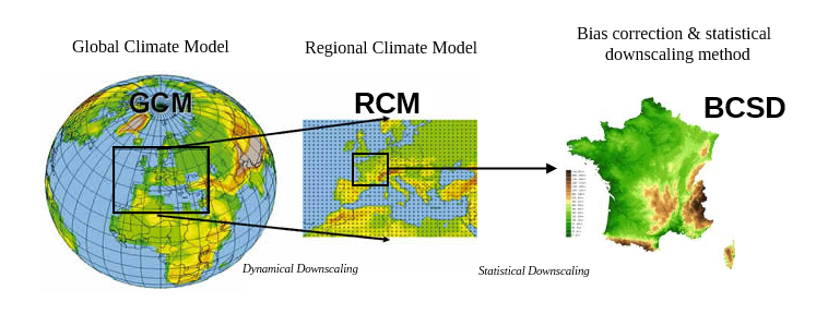
Figure 4.1: Downscaling steps from global to regional modelling to disaggregation at small spatial scales (excerpt from DRIAS2020

For this study, we choose to work with 11 climate projections from the DRIAS2020 data set completed by some projections added for the Explore2 project (Strohmenger, Sauquet, and Thirel, n.d.) forced by RCP 4.5 and 8.5.

The “representative concentration pathways” RCP 4.5 corresponds to a mitigation scenario with a peak of emission by 2040, while the RCP 8.5 corresponds to a “no-policy” scenario with a continuous huge use of fossil fuels (Moss et al. 2010). As shown in Figure 4.2, these 2 emission scenarios are the more likely to happen considering the current trajectory of historical emissions.

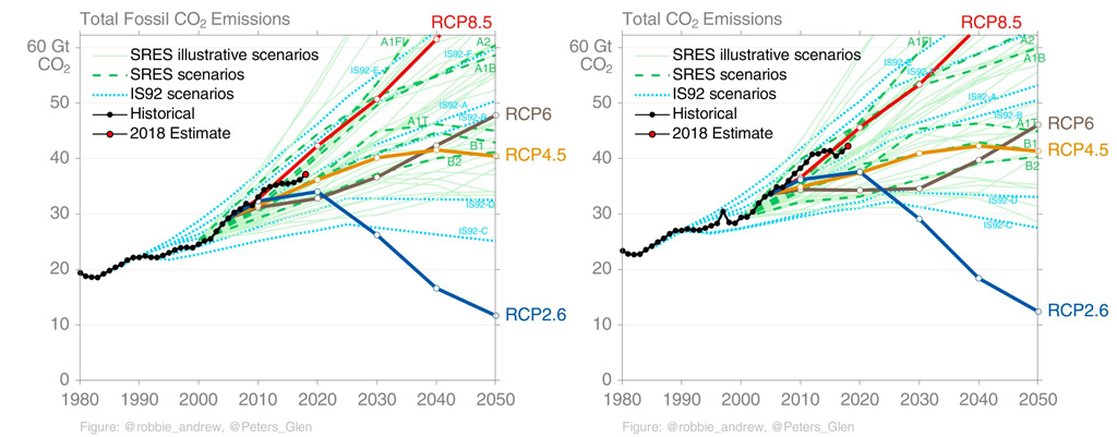
Figure 4.2: Global fossil fuel CO2 emissions (left) and total CO2 emissions from fossil fuels and land use (right) for historical observations and RCP, SRES, and IS92 scenarios. Credit: Glen Peters.

Recently, there was a debate on the opportunity to continue to use RCP 8.5 in prospective studies, because of its weak probability to happen (Ritchie and Dowlatabadi 2017). However, Schwalm, Glendon, and Duffy (2020) argue that not only are the emissions consistent with RCP8.5 in close agreement with historical total cumulative CO2 emissions (within 1%), but RCP8.5 is also the best match out to mid-century under current and stated policies with still highly plausible levels of CO2 emissions in 2100.

Even if the climate projection data set available for the Explore2 project has more climate projections, since we wanted to have the same projections for each RCP in order to make them comparable, the number of available common scenarios was limited to 11 (Table 4.1).

Table 4.1: Climate projections used for the climate change impact assessment

GCM	RCM
CNRM-CERFACS-CNRM-CM5	CNRM-ALADIN63
CNRM-CERFACS-CNRM-CM5	KNMI-RACMO22E
ICHEC-EC-EARTH	KNMI-RACMO22E
ICHEC-EC-EARTH	SMHI-RCA4
IPSL-IPSL-CM5A-MR	IPSL-WRF381P
IPSL-IPSL-CM5A-MR	SMHI-RCA4
MOHC-HadGEM2-ES	CLMcom-CCLM4-8-17
MPI-M-MPI-ESM-LR	CLMcom-CCLM4-8-17
MPI-M-MPI-ESM-LR	MPI-CSC-REMO2009
NCC-NorESM1-M	DMI-HIRHAM5
NCC-NorESM1-M	GERICS-REMO2015

The DRIAS2020 project defines 4 periods for assessing the climate change impact:

• current climate reference (1976-2005): This is a standard period of 30 years of the recent past, which corresponds to the most recent 30-year period possible in the historical simulations and the current reference used in the DRIAS portal.
• near future (2021-2050)
• medium-term future (2041-2070)
• distant future (2071-2100)

We use these periods for assessing the climate change impact through the evolution of hydrological indicators.

4.2 Calculation of the intersection of SAFRAN meshes with the contour of intermediate catchment areas

The Figure 4.3 illustrates the intersection between the cells of the 8x8 km SAFRAN grid and the Seine River intermediate sub-basins of the seinebasin2 model.

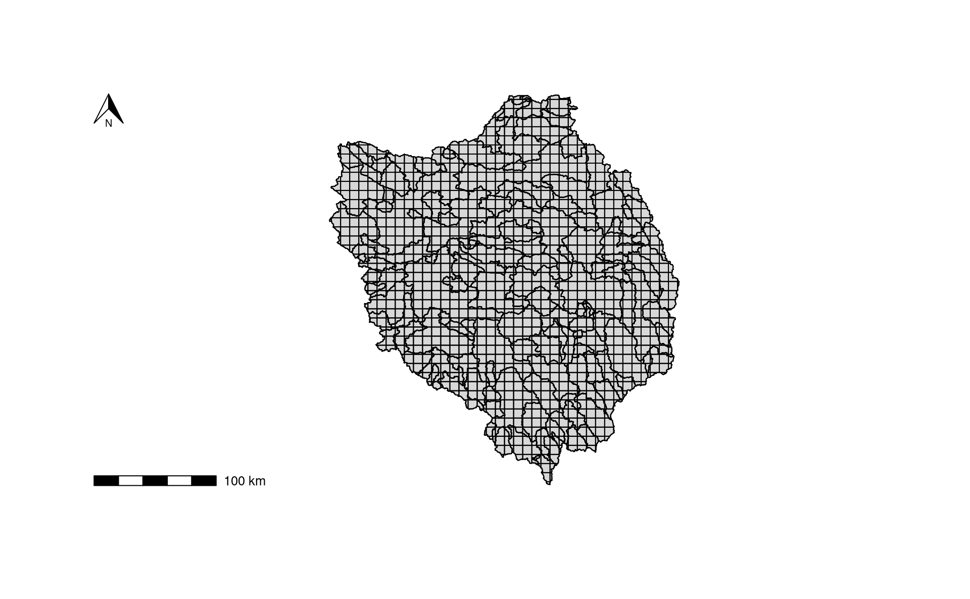
Figure 4.3: Merging of the SAFRAN layer with that of the intermediate catchment areas of the Seine catchment at Vernon

For each intermediate sub-basin, we compute which cells and proportion of them are concerned in order to compute the mean meteorological data at this scale. The Table 4.2 shows an excerpt of the resulting conversion table with \(x\) and \(y\) the coordinates of the SAFRAN cell centroid, \(CODE\) the gauging station identifier, \(area\) the area of the intersection in km², and \(prop\) the proportion of the intersection area compared to the sub-basin area.

Table 4.2: Conversion table for aggregating meteorological data at the intermediate sub-basin scale

x	y	CODE	area	prop
820000	2449000	H6102010	6.112018	0.0216247
828000	2417000	H6102010	18.732000	0.0662751
828000	2425000	H6102010	27.565881	0.0975300
828000	2433000	H6102010	10.824818	0.0382990
828000	2441000	H6102010	0.233000	0.0008244
820000	2345000	H5042010	2.560719	0.0151647
820000	2353000	H5042010	19.777100	0.1171213
820000	2361000	H5042010	12.243082	0.0725043
828000	2337000	H5042010	2.339519	0.0138548
828000	2345000	H5042010	57.788381	0.3422266
828000	2353000	H5042010	47.727632	0.2826462
828000	2361000	H5042010	6.433868	0.0381018
836000	2337000	H5042010	2.882932	0.0170729
836000	2345000	H5042010	14.895000	0.0882092
836000	2353000	H5042010	2.211768	0.0130982

4.3 Climate projection bias at the intermediate sub-basin scale

The climate projections has been unbiaised by the ADAMONT method (Verfaillie et al. 2017) and are supposed to produce a similar climate than the one historically observed over the past period (1950-2005).

The Figures 4.4, 4.5, and 4.6 show respectively the correspondence of the monthly mean precipitation, daily mean temperature, and potential evaporation between historical observations and climate projections over the reference period (1976-2005). Climate projections of temperature and potential evaporation match very well with historical data. Results on precipitation is a bit more spreaded, this is due to the fact that rainfall events can be very localized in space and time and that can have a big influence on the mean monthly precipitation especially if we considere that the Paris sub-basin area is relatively small (536 km²). Nevertheless, all climate projections are converging around historical value at the year scale and the general monthly trend is respected.

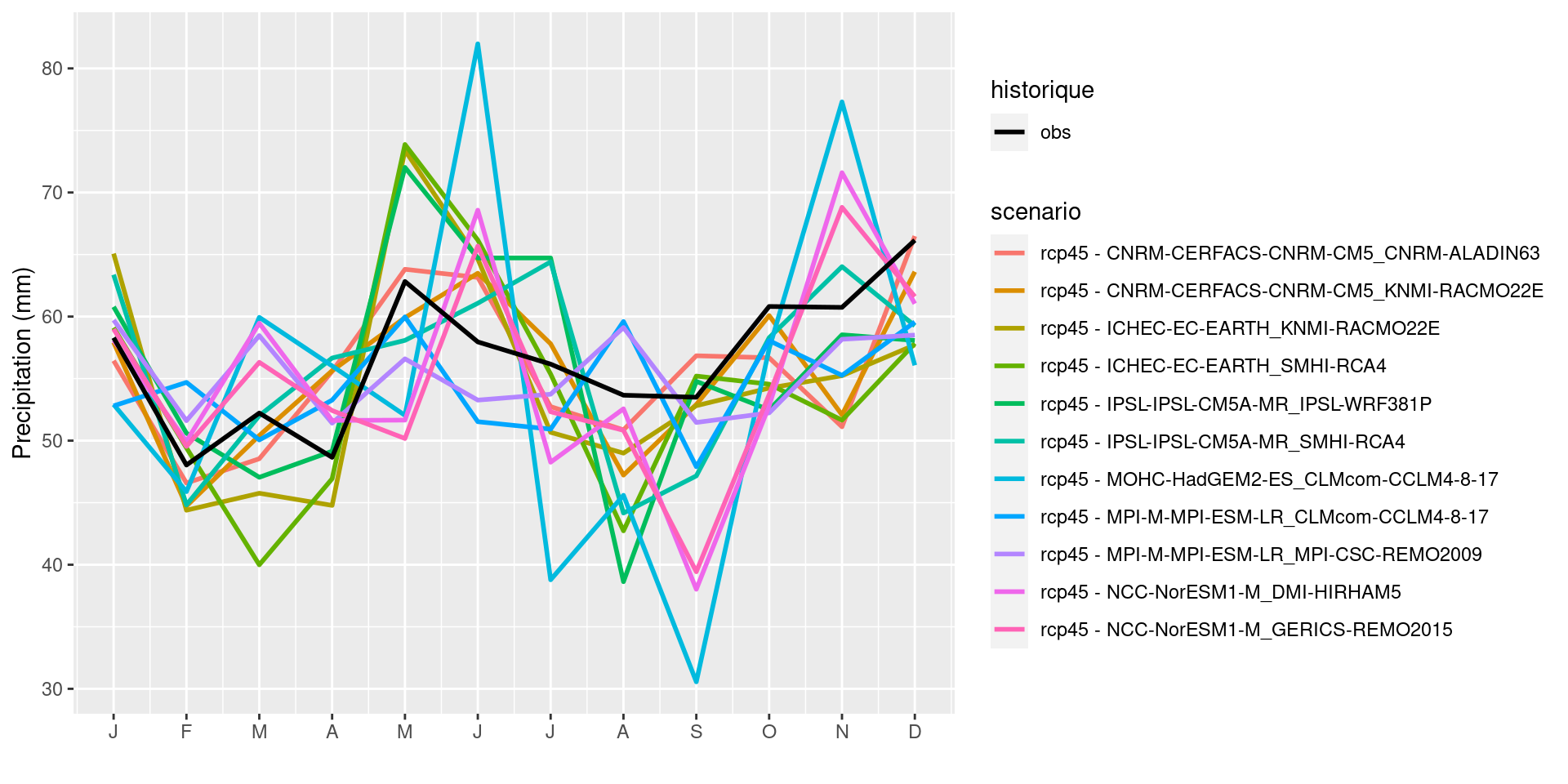
Figure 4.4: Monthly mean precipitation for the intermediate sub-basin at Paris (H5920010) calculated on period 1976-2005: comparison between observations and climate projections

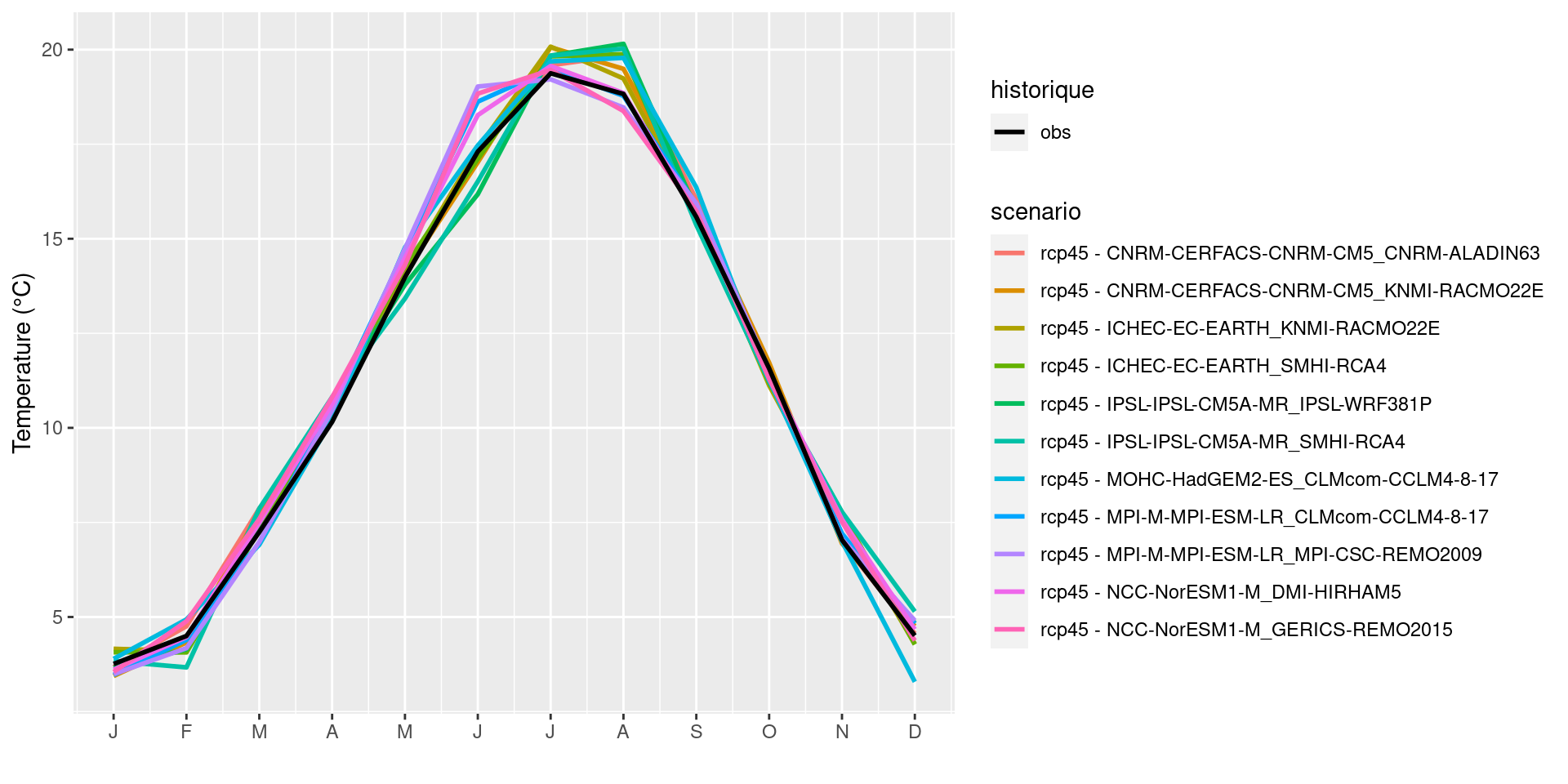
Figure 4.5: Monthly mean daily temperature for the intermediate sub-basin at Paris (H5920010) calculated on period 1976-2005: comparison between observations and climate projections

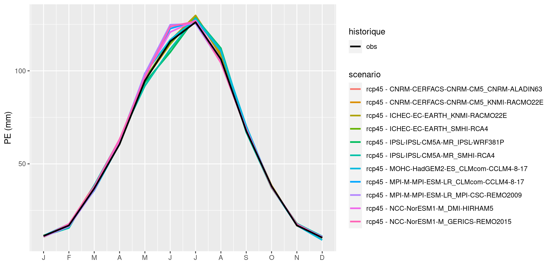
Figure 4.6: Monthly mean potential evaporation for the intermediate sub-basin at Paris (H5920010) calculated on period 1976-2005: comparison between observations and climate projections

References

Moss, Richard H., Jae A. Edmonds, Kathy A. Hibbard, Martin R. Manning, Steven K. Rose, Detlef P. van Vuuren, Timothy R. Carter, et al. 2010. “The Next Generation of Scenarios for Climate Change Research and Assessment.” Nature 463 (7282, 7282): 747–56. https://doi.org/10.1038/nature08823.

Ritchie, Justin, and Hadi Dowlatabadi. 2017. “Why Do Climate Change Scenarios Return to Coal?” Energy 140 (December): 1276–91. https://doi.org/10.1016/j.energy.2017.08.083.

Schwalm, Christopher R., Spencer Glendon, and Philip B. Duffy. 2020. “RCP8.5 Tracks Cumulative CO2 Emissions.” Proceedings of the National Academy of Sciences 117 (33): 19656–57. https://doi.org/10.1073/pnas.2007117117.

Strohmenger, Laurent, Eric Sauquet, and Guillaume Thirel. n.d. “Explore2: Les Futurs de l’eau.”

Verfaillie, Deborah, Michel Déqué, Samuel Morin, and Matthieu Lafaysse. 2017. “The Method ADAMONT V1.0 for Statistical Adjustment of Climate Projections Applicable to Energy Balance Land Surface Models.” Geoscientific Model Development 10 (11): 4257–83. https://doi.org/10.5194/gmd-10-4257-2017.

Vidal, Jean-Philippe, Eric Martin, Laurent Franchistéguy, Martine Baillon, and Jean-Michel Soubeyroux. 2010. “A 50-Year High-Resolution Atmospheric Reanalysis over France with the Safran System.” International Journal of Climatology 30 (11): 1627–44. https://doi.org/10.1002/joc.2003.