Chapter 3 Calibration of the model
3.1 Model input
The semi-distributed hydrological model requires input climate data for the calibration process. On each intermediate sub-catchment (Figure 2.1), it uses precipitation, potential evaporation, and temperature. Precipitation and temperature data are extracted from the SAFRAN reanalysis database (Vidal et al. 2010). The potential evapotranspiration is calculated from the Oudin formula (Oudin et al. 2005) which only uses temperature, day of the year and geographical latitude as inputs.
For the calibration, we use the complete data set available between the 1st of August 1958 and the 31th of July 2022 at daily time step.
Observed flow data used for calibration are extracted from the HYDRO database using HYDRO3 station codes for each of the 152 stations in the study (Leleu et al. 2014). We use all available data also between 1958 and 2022.
The intake and release flow data observed for the 4 reservoir lakes are extracted from the daily operating files supplied by the ETPB Seine Grands Lacs. These data will be used to take into account the influence of the reservoir lakes on river flows.
3.2 Calibration of basin stations with the addition of reservoirs and diversions
The model contains a schematic representation of the river network in which, each intermediate sub-catchment is represented by a node used by the airGRiwrm package.
3.2.1 Adjustment of the natural hydrological network to integrate Reservoir and Diversion nodes
A modification to the network present in the GRiwrm object is required to incorporate the reservoir influences.
The airGRiwrm extension used in seinebasin2 allows various nodes to be added:
- the
Reservoirnode allows you to model the volume evolution of a reservoir from one or more upstream nodes for filling and one downstream node for the release (release time series provided by the user); - the
Diversionnode allows to divert water from an existing node to another (diversion time series provided by the user); - the
Ungaugednode, allows to simulate the flow on the river network on a location not equipped by a gauging station by copying hydrological parameters from a downstream gauged node thanks to a common calibration.
All the Seine basin reservoirs can be conceptualized as in Figure 3.1. All the reservoirs have one river outlet that controls the release of the reservoir. A reservoir can be a dam across the river such as for the Pannecière Lake (Yonne River), and in this case, it doesn’t have river inlets that control the filling. Other reservoir on the Seine basin are derived with one or several river inlets (denoted as river intlet i in Figure 3.1). Marne and Seine lakes don’t have natural impluvium which is not the case for the Yonne lake naturally filled by the Yonne river, and the Aube lake naturally filled by the Auzon and the Amance rivers. Finally, the Marne and the Aube lakes replenish former rivers that have been cut at the reservoir construction. These replenishment are processed independently from other reservoir rules even if this flow is added to the reservoir release in the model.
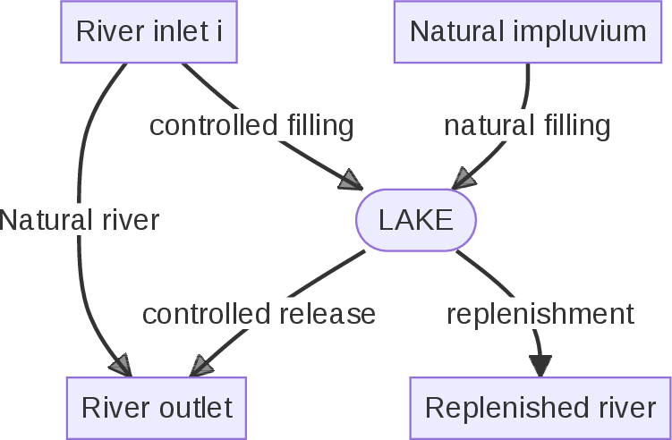
Figure 3.1: Conceptual scheme of reservoir connections with the river system
The Seine implementation of the Seine reservoir is represented in Figures 3.2 and 3.3.
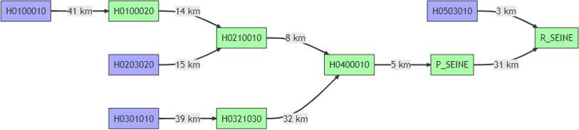
Figure 3.2: Diagram of natural network around the lake Seine
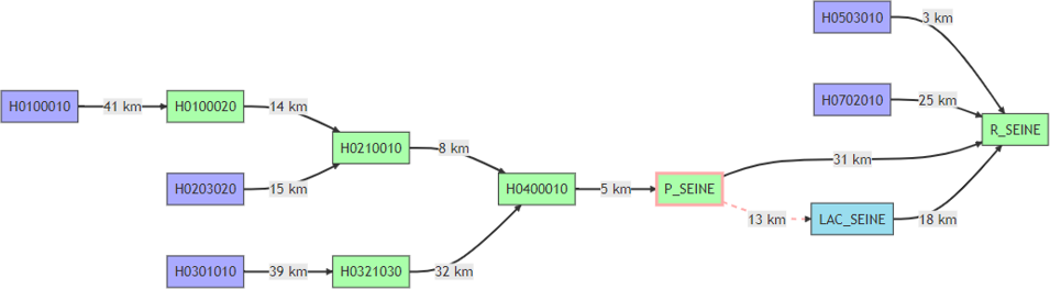
Figure 3.3: Diagram of the network around the lake Seine after reservoir implementation
The Yonne lake, as an inline reservoir, is not complicated to implement as we can see in Figures 3.4 and 3.5.

Figure 3.4: Diagram of natural network around the lake Yonne

Figure 3.5: Diagram of the network around the lake Yonne after reservoir implementation
The Marne lake is provided with 2 inlets on the Marne and Blaise rivers with one outlet
(Figure 3.6). The reservoir is partly located on the Aube watershed
through the replenishment of the Droyes River which flows to the intermediate sub-catchment
“L’Aube à Arcis-sur-Aube” (H1501010). The implementation of the Marne reservoir is represented
in Figure 3.8.
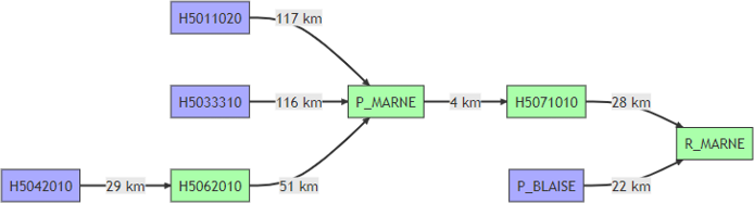
Figure 3.6: Diagram of natural network around the lake Marne
The Aube reservoir presents a specific context (Figure 3.7).
This reservoir is made up of two smaller reservoirs,
Lake Auzon-Temple and Lake Amance which, are linked by an open canal and
are located on two distinct river basins.
The first feeds the Auzon river, whose downstream basin is “L’Aube à Arcis-sur-Aube” (H1501010).
The second feeds the Amance, whose downtream basin is R_AUBE the release point
of the reservoir in the Aube River.
The model mimics this behaviour until 1988 when the reservoir was built.
After this date all the flow from the Auzon and Amance rivers is diverted to the
reservoir and the replenishment flow for the Auzon river is diverted from R_AUBE
to the gauging station H1501010 as illustrated in the Figure 3.8.
As the AMANCE and AUZON have no observed flows, we define them as Ungauged.
This means that these sub basins are calibrated with and will use parameters derived from
the nearest downstream gauged basin, in this case R_AUBE, to simulate flows.
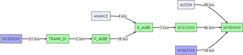
Figure 3.7: Diagram of natural network around the lake Aube
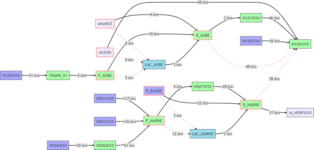
Figure 3.8: Diagram of the network around the lake Aube and Marne after reservoir implementation
Observed flows at inlets and outlets of the reservoirs are injected in the model through
the Diversion and Reservoir nodes in order to process to the calibration using
influenced observed flows.
3.2.2 Calibration of the 152 stations in the study area, taking reservoirs into account
The calibration process computes the optimized parameters for each catchment.
The AMANCE and AUZON nodes, are defined as Ungauged because no observed flow is available
to calibrate these catchments. The calibration is then performed following the method “M2”
developed by Lobligeois (2014). This calibration consists in defining
a “donor” node which has observed flows and is calibrated together with the ungauged node.
Hydrological model parameters are copied from the donor to the ungauged node with the exception that the unit hydrograph parameter \(X4\) depends on the area of the sub-catchment following Equation (3.1).
\[\begin{equation} x_{4i} = \left( \dfrac{S_i}{S_{BV}} \right) ^ {0.3} X_4\tag{3.1} \end{equation}\]
The airGRiwrm package natively defines a “donor” for each node in the network.
By default, it assigns the first downstream gauged node as donor.
As one can see on Figure 3.7, The AMANCE node has the R_AUBE node as donor and
the AUZON node should have the H1501010 node as donor. But the implementation,
of the reservoir (Figure 3.8) adds a connection between the AUZON node
and the R_AUBE node through the reservoir. This creates a conflict because
H1501010 and R_AUBE become interdependent and should be calibrated all together which
is currently not possible. Therefore, we have chosen as well to define R_AUBE as donor for
the ungauged AUZON node.
The calibration consists in finding the model parameters which optimized a performance criterion. We use here a composite criterion containing a parameter regularization as defined by de Lavenne et al. (2019) which adds a priori information on optimal parameter sets for each modeling unit of the semi-distributed model. Calibration iterations are then performed by jointly maximizing simulation performance and minimizing drifts from the a priori parameter sets.
As proposed by de Lavenne et al. (2019), we use the Kling-Gupta Efficiency (KGE) criterion (Gupta et al. 2009) (Equation (3.2)) calculated on the square root of the discharge.
\[\begin{equation} KGE = 1 - \sqrt{(r - 1)^2 + (\alpha - 1)^2 + (\beta - 1)^2}\tag{3.2} \end{equation}\]
- \(\alpha\) : Ratio of simulated and observed flow variances
- \(\beta\) : Model bias
- \(r\) : Correlation coefficient between observed and simulated flow rates
This criterion is used to quantify a bias between observed flow values and simulated model output values. This criterion varies between -inf and 1, and the closer it is to 1, the smaller the difference between the simulated and observed values.
3.3 Simulation for all intermediate bassin in influenced context
The maps below show the spatial variability of the four parameters defined during the calibration process with reservoir influence:
- \(x_1\) corresponds to the maximum capacity of the production reservoir (mm);
- \(x_2\) corresponds to the loss/gain coefficient due to inter-basin exchanges at the underground level (mm/d);
- \(x_3\) is the capacity at one-time step of the routing reservoir (mm);
- \(x_4\) is the unit hydrograph (day).
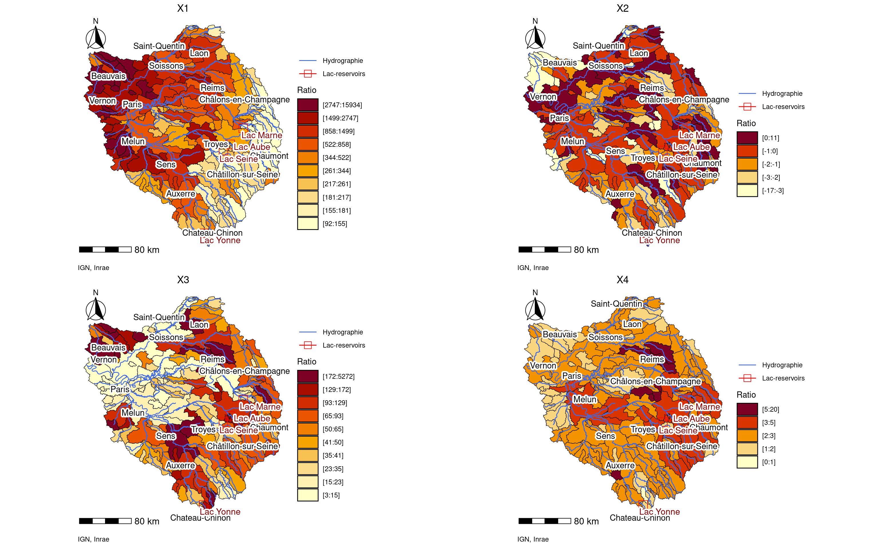
Figure 3.9: Maps of calibration parameters including the influence of the reservoirs
The inclusion of reservoirs in the modelling results in a significant improvement in flow simulation.
Stations H1501010, R_MARNE and R_SEINE show simulated regimes that are closer to those observed.
However, for station H20201010, the simulated flows barely match with observed ones (Figure 3.10).
The simulation is less good during the period from June to November, when the model overestimates the flows.
We didn’t succeed to find out why we get this poor result on this gauging station.
The most probable reason would be a poor rating curve on this gauging station.
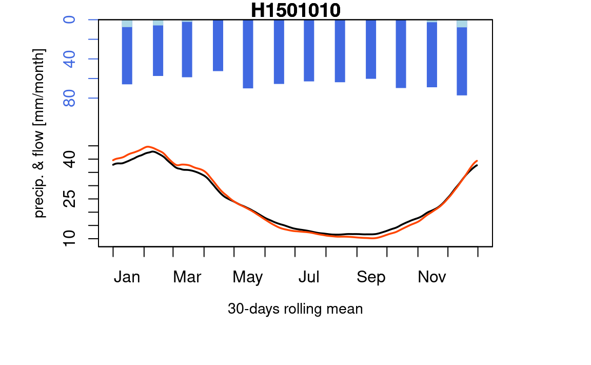
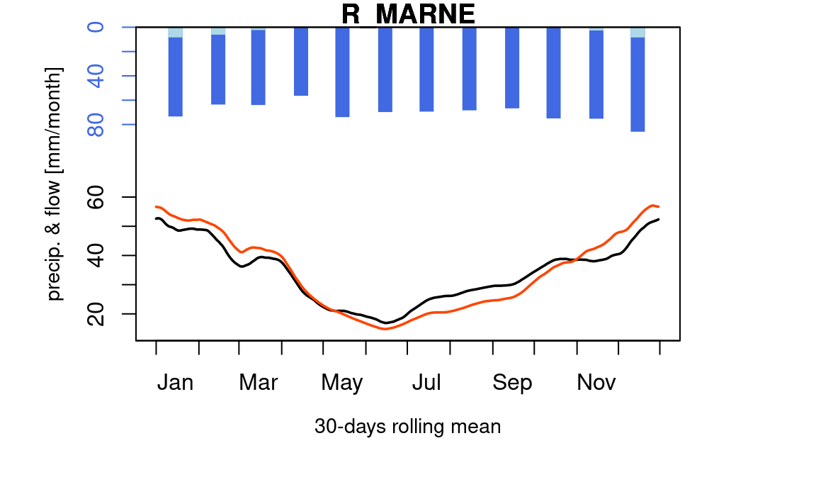
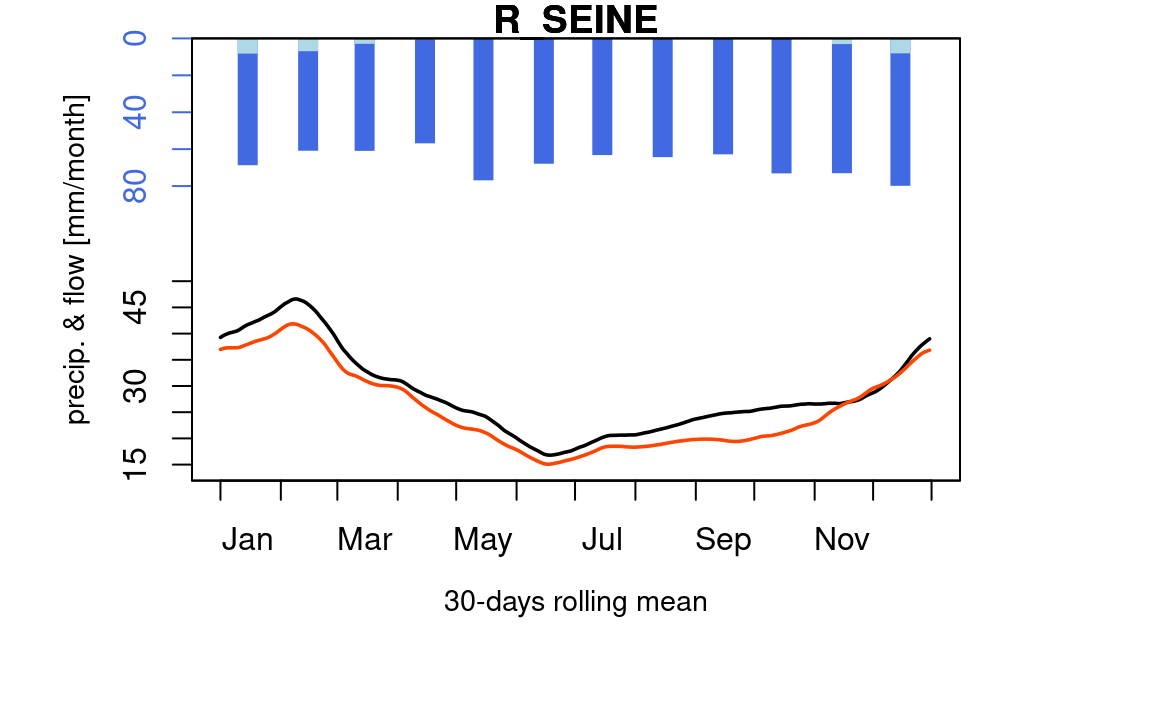
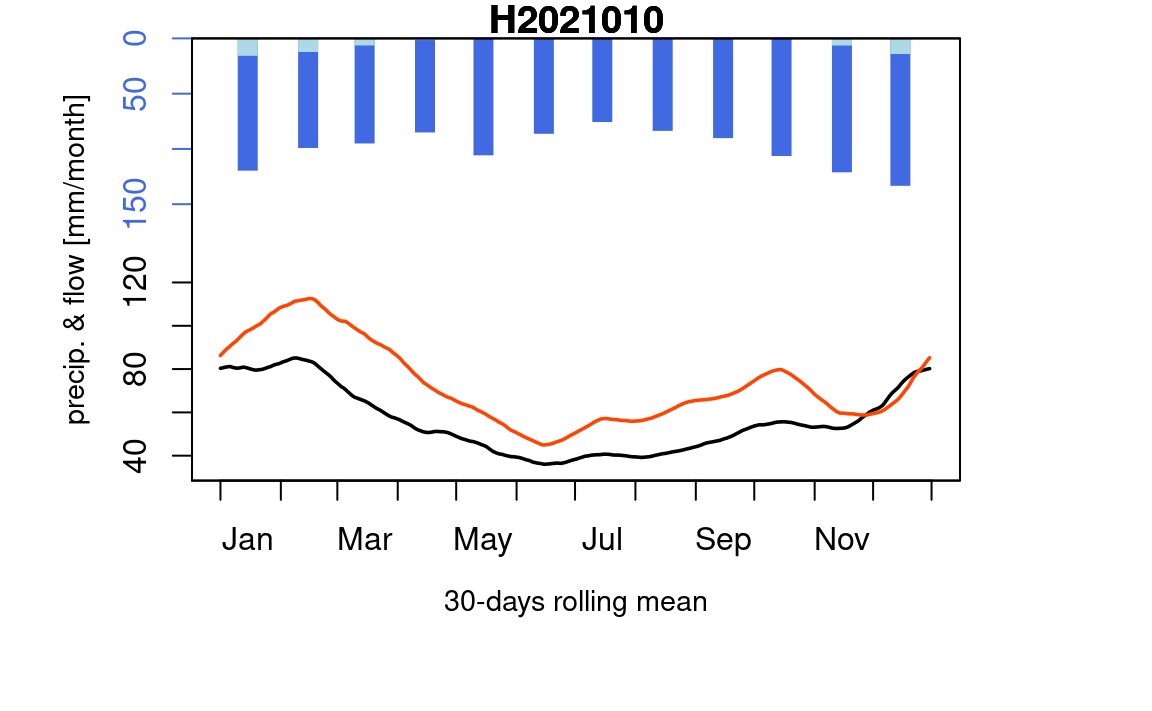
Figure 3.10: Simulated and observed flow regimes incorporating the influence of reservoirs
For each station, a summary sheet of the flow, rainfall and regime records used for calibration is recorded and available here: https://nextcloud.inrae.fr/s/dweGCFJoke5R6qc
3.4 Model performance evaluation
We use the Kling-Gupta Effiency (KGE) criterion defined in Equation (3.2) calculated from the output of the simulation with reservoir influence in order to evaluate the results of the model taking into account the influence of the four reservoir lakes.
For most of the intermediate basins, the KGE criterion is between 0.8 and 1 (Figure 3.11) which reflects a accurate representation of observed flows. The “no data” areas correspond to the Amance and Auzon sub basins where the KGE indicator cannot be calculated because of the lack of observed flows.
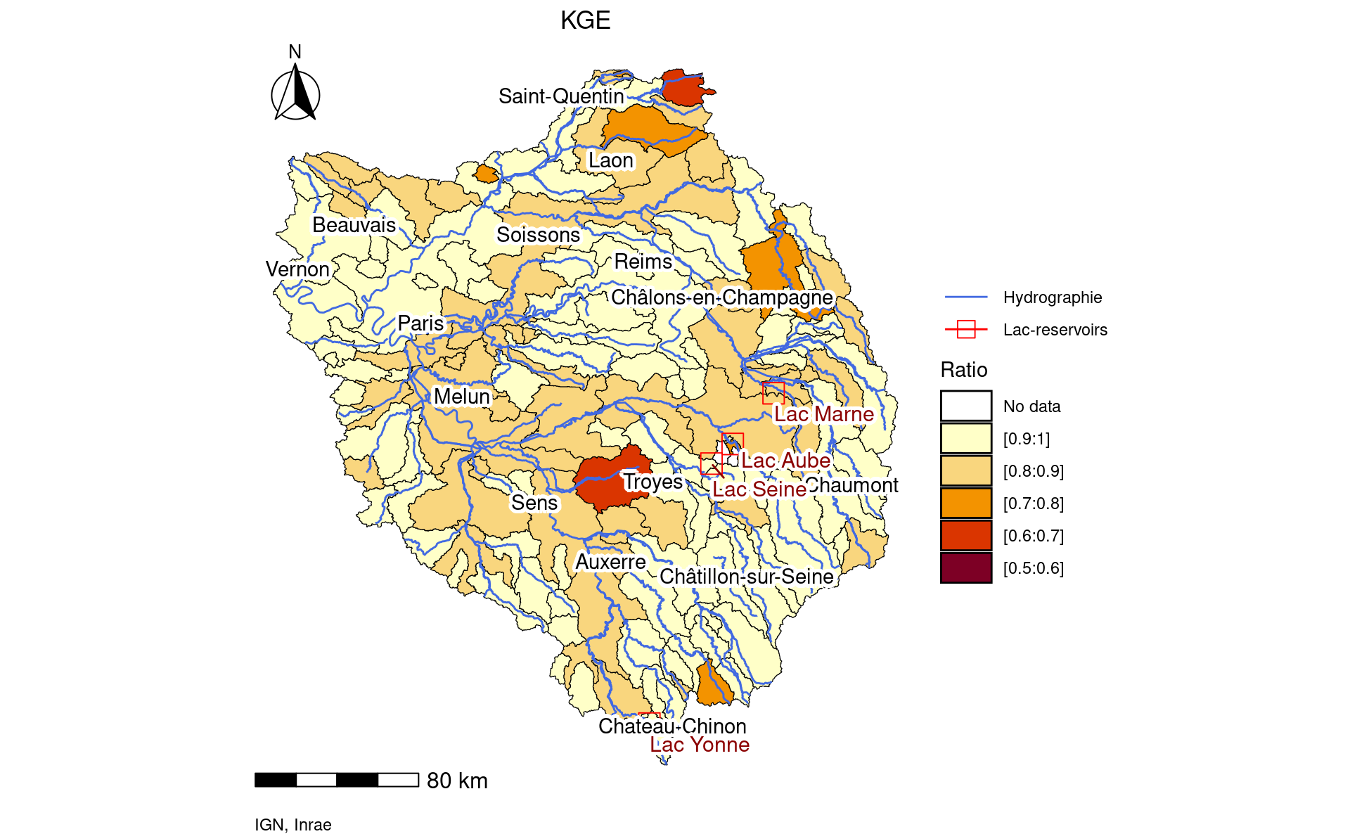
Figure 3.11: Maps of KGE criteria for calibration with the integration of the influence of reservoirs
The simulation performances are also assessed with hydrological indicators related to mean flow, high-flows and low-flows. We here use such indicators already used in the explore 2070 project (Chazot et al. 2012):
- The mean annual discharge “QA” provides a general measure of the quantity of water flowing over a year.
- The “VCN10” and “VCN30” low-flow indicators are respectively the average minimum flows over periods of 10 and 30 consecutive days.
- The “QMNA2” and “QMNA5” low-flow indicators are the lowest average monthly flows over a year with a return period of respectively 2 and 5 years.
- The “QJXA2”, “QJXA10” and “QJXA20” high-flow indicators are the maximum daily flows over a return period of 2, 10 and 20 years respectively.
Low flow indicators are computed from a statistical adjustment of a Galton distribution, and high-flow indicators are computed from a statistical adjustment of a Gumbel distribution.
The accuracy of the models used in the study are assessed from ratios “R-” between these indicators calculated from simulated and observed flows as illustrated in Equation (3.3).
\[\begin{equation} R\textnormal{-}QA = \dfrac{QA_{simulated}}{QA_{observed}} \tag{3.3} \end{equation}\]
The following maps illustrate the ratios calculated between simulated and observed flows for various hydrological indicators in all 152 intermediate catchments except for the AMANCE and AUZON, which have no observed data.
3.4.1 Calibration performance on QA (average flow)
The “R-QA” indicators reflects that the simulated flows produced a good interannual volume of water. It is a key indicator in term of water resource management at annual scale.
In all the intermediate catchments, the values of “R-QA” are generally between 0.9 and 1, which indicates that the annual mean of the simulated flows is similar to the observed flows (Figure 3.12).
This result is not surprising since the mean flow bias is used in the KGE criterion (Equation (3.2)).
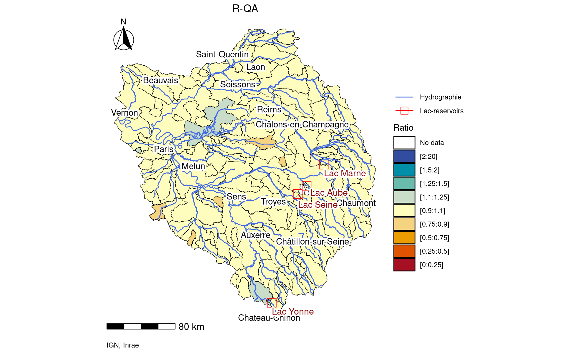
Figure 3.12: Map of R-QA indicators for simulated flows with observed reservoir influences calculated on period 1959-2022
3.4.2 Calibration performance on VCN30 with a 2-year return period
As far as low-flow indicators are concerned, most of the intermediate catchment areas show ratios of between 0.75 and 0.9, suggesting an underestimation of simulated flows of the order of 10 to 25% (Figure 3.13). For the other basins, the ratios vary considerably, sometimes going as far as a very pronounced underestimate (close to 0.25) or a significant overestimate (close to 2) for some upstream basins.
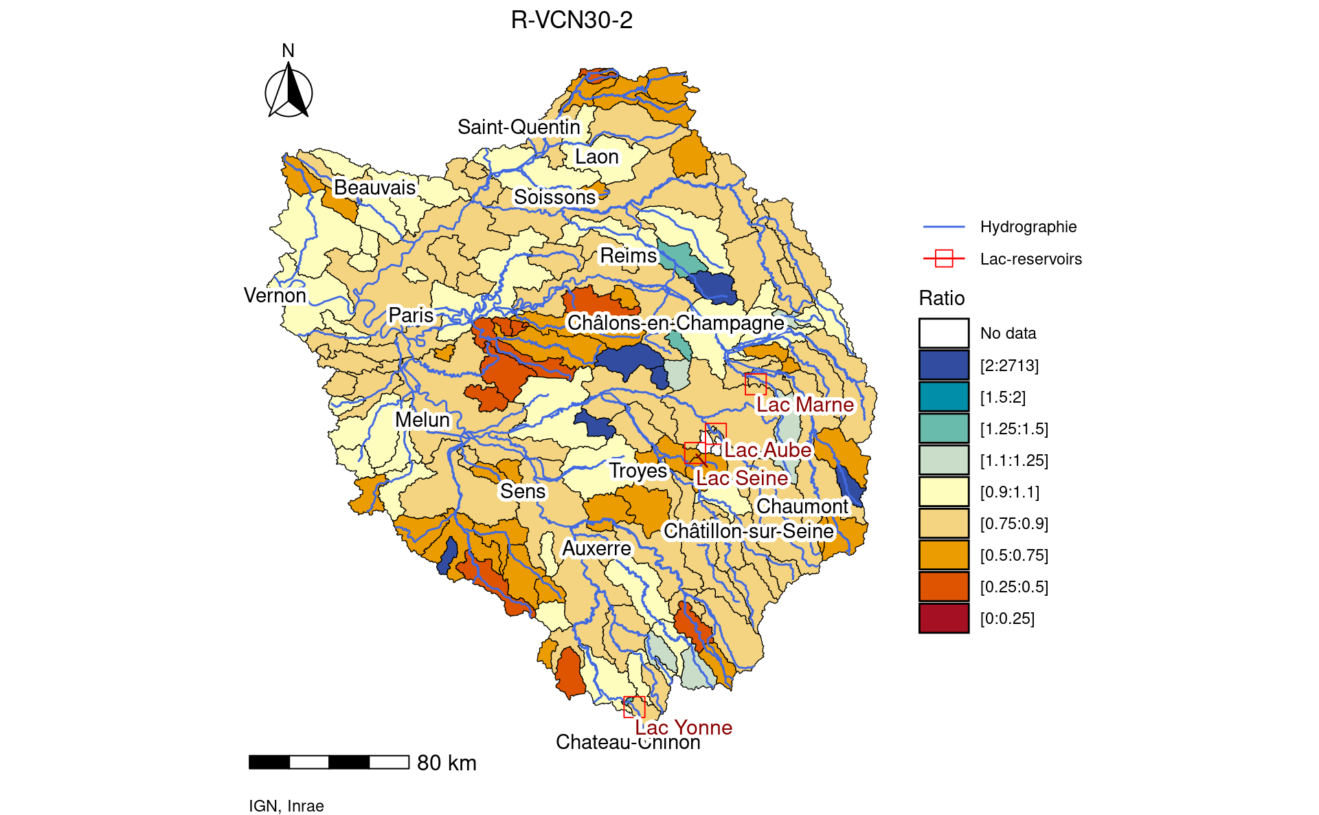
Figure 3.13: Map of R-VCN30-2 indicators for simulated flows with observed reservoir influences calculated on period 1959-2022
3.4.3 Calibration performance on QMNA5
The Figure 3.14 shows the map of the “R-QMNA5” ratios. These results are quiet similar as those obtained on the “R-VCN30-2” ratios.
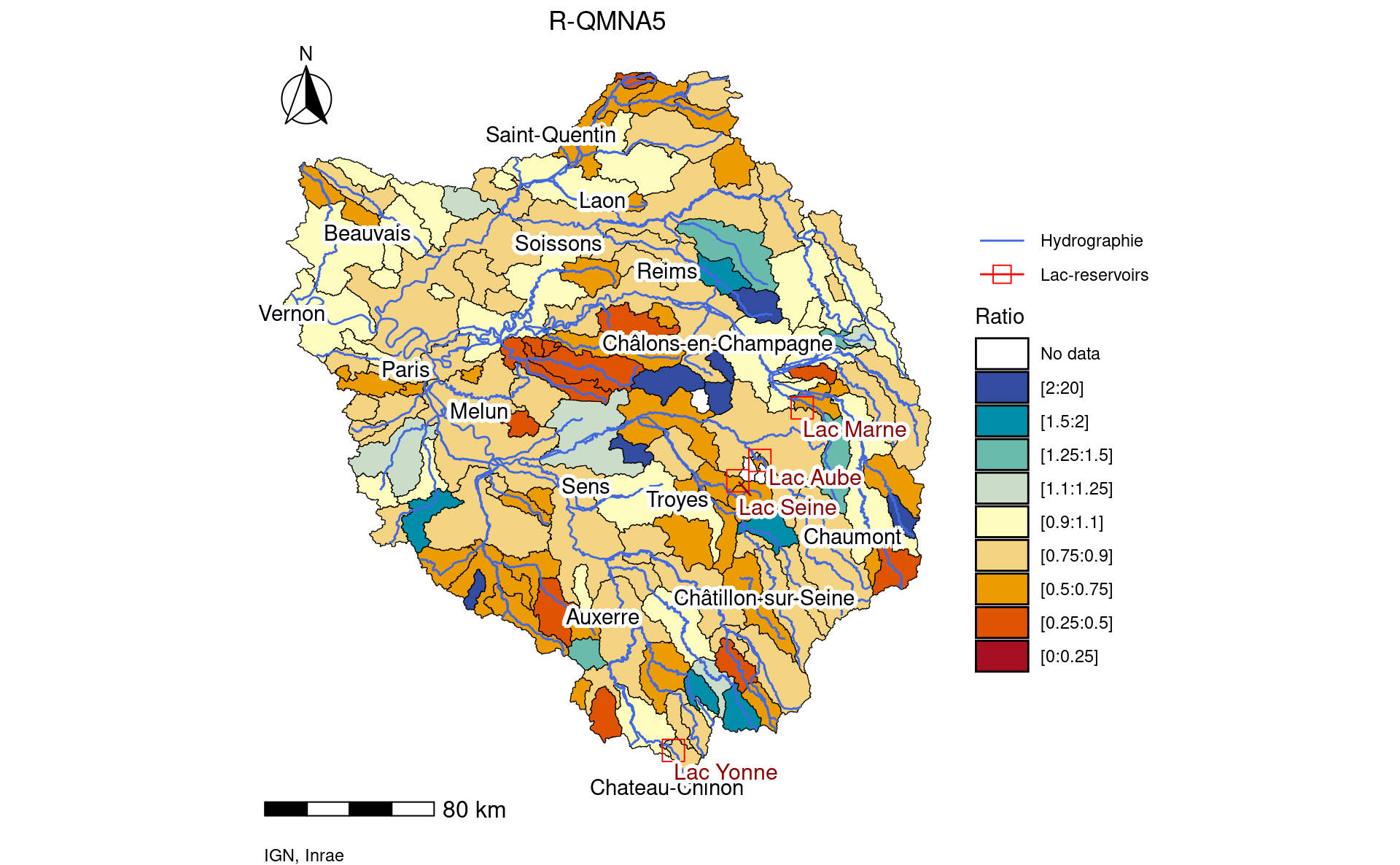
Figure 3.14: Map of R-QMNA5 indicators for simulated flows with observed reservoir influences calculated on period 1959-2022
3.4.4 Calibration performance on QJXA10
For maximum daily flows with a 10-year return period, the ratios are generally between 0.75 and 1.5.
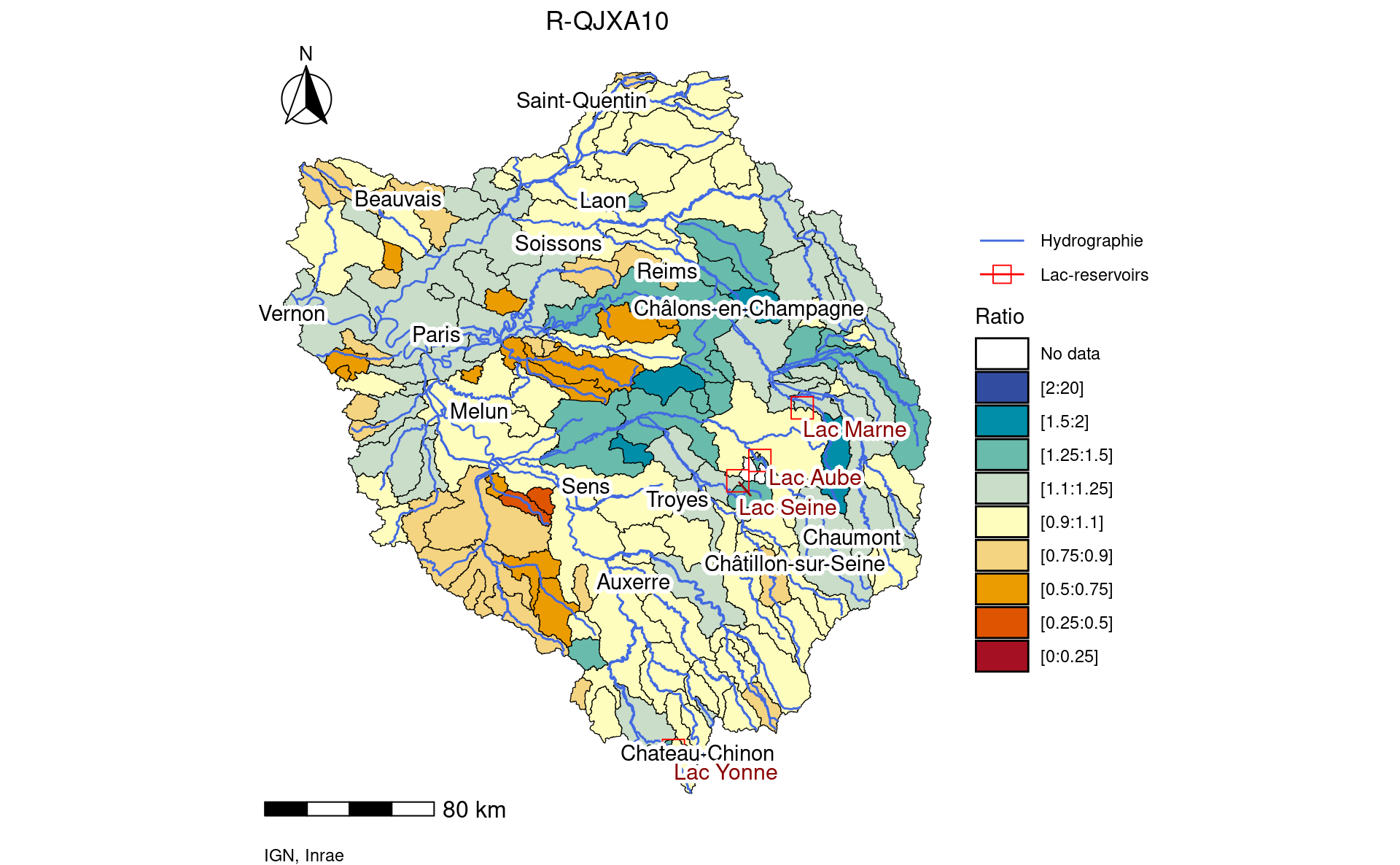
Figure 3.15: Map of R-QJXA10 indicators for simulated flows with observed reservoir influences calculated on period 1959-2022
3.4.5 Overview of all calibration performance indicators
We highlight 9 hydrometric stations used as monitoring stations for the assessment of the reservoir management performance (Dorchies et al. 2014). The spider diagram below shows all the hydrological indicator ratios for these stations.
Of the nine stations, the model underestimates the simulated flows for low-flows (“VCN” and “QMNA” indicators) at seven of them (by an average of 0.75). Only the COURL and ALFOR stations reproduce the data accurately.
For high flows (“QJXA” indicators), the ARCIS station is clearly underestimated, while the other stations are around 1, with the exception of the COURL, ALFOR and CHALO stations, which are overestimated by around 25%. The NOGEN station is the most overestimated, approaching 30%.
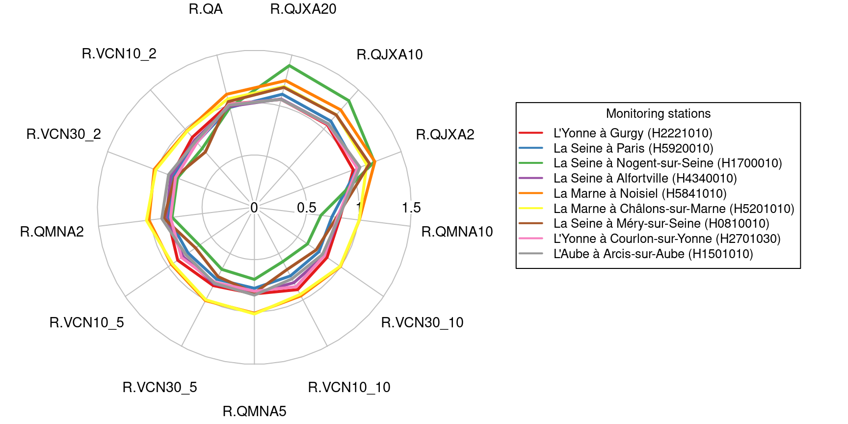
Figure 3.16: Ratio between hydrological indicators calculated on simulated and observed influenced flows on the period 1959-2022
Hydrological indicators for observed and simulated flows are recorded here in the same format as will be used to analyse historical and projected natural flows.
These indicators can be downloaded from : https://nextcloud.inrae.fr/s/adinzGa3AmLEXnZ/download?path=%2F02-calibration&files=Q_indicators_with.tsv